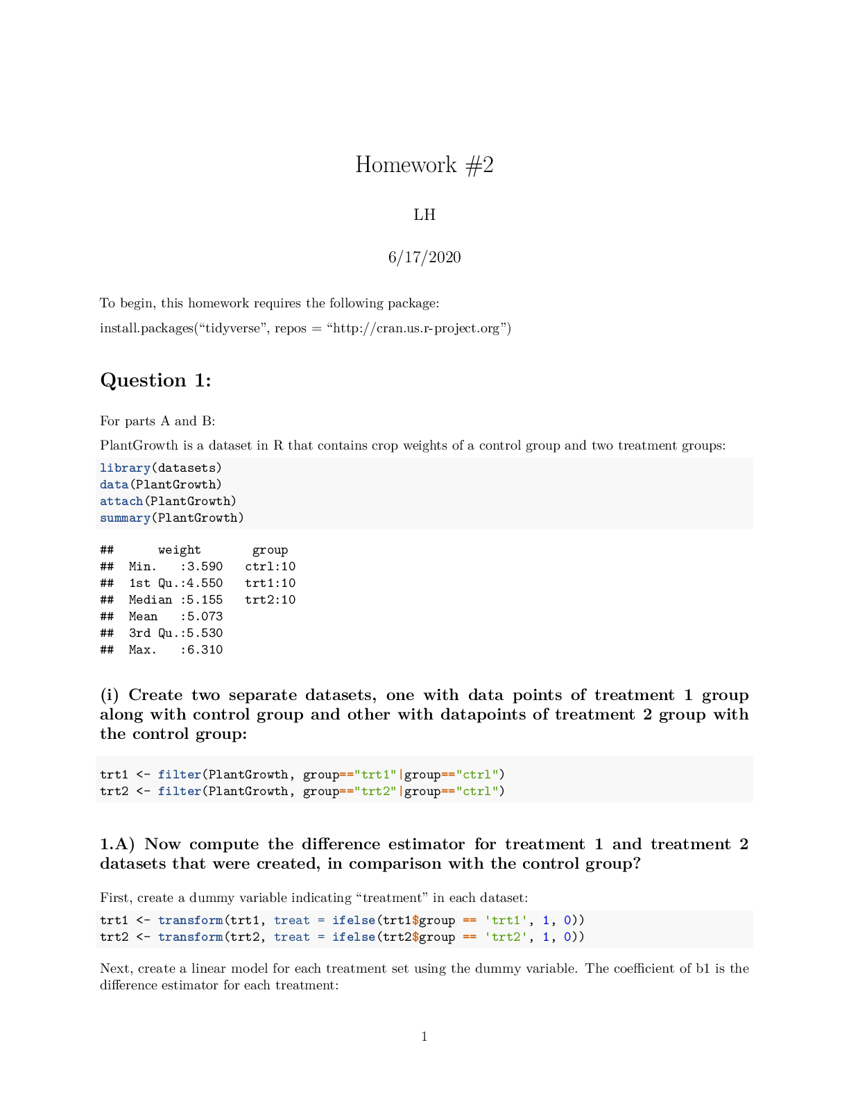
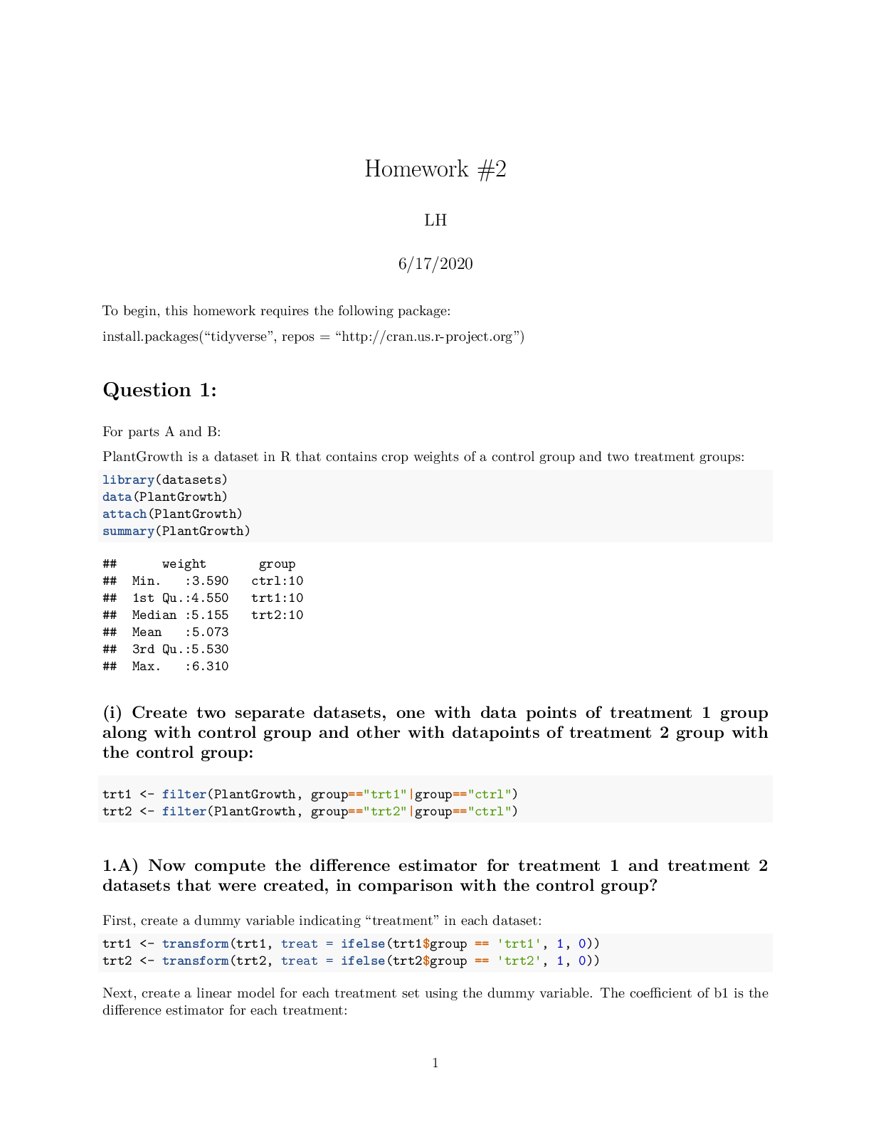
PlantGrowth is a dataset in R that contains crop weights of a control group and two treatment groups:
library(datasets)
data(PlantGrowth)
attach(PlantGrowth)
summary(PlantGrowth)
## weight group
## Min. :3.590 ctrl:10
## 1st Qu.:4.550 trt1:10
## Median :5.155 trt2:10
## Mean :5.073
## 3rd Qu.:5.530
## Max. :6.310
(i) Create two separate datasets, one with data points of treatment 1 group
along with control group and other with datapoints of treatment 2 group with
the control group:
trt1 <- filter(PlantGrowth, group=="trt1"|group=="ctrl")
trt2 <- filter(PlantGrowth, group=="trt2"|group=="ctrl")
1.A) Now compute the difference estimator for treatment 1 and treatment 2
datasets that were created, in comparison with the control group?
First, create a dummy variable indicating “treatment” in each dataset:
trt1 <- transform(trt1, treat = ifelse(trt1$group == 'trt1', 1, 0))
trt2 <- transform(trt2, treat = ifelse(trt2$group == 'trt2', 1, 0))
Next, create a linear model for each treatment set using the dummy variable. The coefficient of b1 is the
difference estimator for each treatment:
1
#Treatment 1 Model:
lm.trt1 <- lm(weight ~ group, data = trt1)
summary(lm.trt1)$coefficients
## Estimate Std. Error t value Pr(>|t|)
## (Intercept) 5.032 0.2202177 22.85012 9.547128e-15
## grouptrt1 -0.371 0.3114349 -1.19126 2.490232e-01
The difference estimator for treatment 1 is -0.371.
#Treatment 2 Model:
lm.trt2 <- lm(weight ~ group, data = trt2)
summary(lm.trt2)$coefficients
## Estimate Std. Error t value Pr(>|t|)
## (Intercept) 5.032 0.1636867 30.74166 5.206846e-17
## grouptrt2 0.494 0.2314879 2.13402 4.685138e-02
The difference estimator for treatment 2 is 0.494.
1.B) From the PlantGrowth dataset what is the average crop weight of the
control group, treatment 1 group, and treatment 2 group, comment on which
group has the highest average?
The mean of the control group is the intercept of either model, which is equal to _5.032__.
The mean of the treament 1 group can be calulated by: Diff. Est. + Control Mean = Treatment 1 Mean
summary(lm.trt1)$coefficients[2] + summary(lm.trt1)$coefficients[1]
## [1] 4.661
Likewise to find the mean of the treatment 2 group:
summary(lm.trt2)$coefficients[2] + summary(lm.trt2)$coefficients[1]
## [1] 5.526
The treatment 2 group had the highest average weight (5.526), which means that the plants grew the most
due to the experimental “treatment” than both the control group and the treatment 1 group. This treatment
could be the type or amount of fertilizer applied applied to the treatment 2 group, for example.
(Note that treatment 1 group had a lower average (4.661) than the control group, which means that the
treatment applied actually resulted in less growth than the control group.)
For parts C, D, and E: using the dataset Min_Wage.csv
Read More


